Let’s Learn A Trick in MS Excel with Monika
Learning in GreyB is a perpetual process. Everyone make sure that his/her colleague or junior should possess the best knowledge of the domain.
Here in GreyB, we have multiple teams with their own expertise. One team can teach another a thing or two. The conventional method says to arrange a workshop where one team teaches a skill to the rest. That, however, is not that effective. Why you ask? I’ll quote Benjamin Franklin as my answer.
Tell me and I forget. Teach me and I remember. Involve me and I learn.
You may have sensed that we want everyone to learn a thing by not teaching them but by involving them. With that in mind, we started a learning activity series in which a member of a particular team organizes on email. And everyone is given 10 minutes to reply with a solution.
To give you an example, here I am sharing one of the activities conducted by Monika Chadha, a senior associate from our Graphical Team.
So, here’s what Monika shared during first few seconds of those enthralling ten minutes:
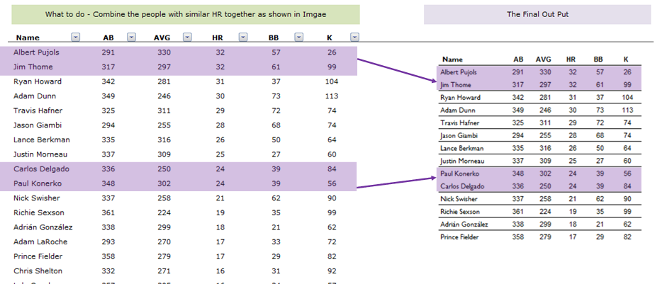
You are given a table with sample data. The purpose is to put borders between the rows of a table. But, here’s a catch. You’re not allowed to use “add border” option. Also, there shouldn’t be a border between rows where a value repeats in the “HR” column.
The image below will help you understand:
Hint: Here I have a hint for you to make the task bit easy. Conditional formatting. And Google search, of course.
A Holy Rule: You need to send the screenshots of steps that help you find the solution.
Within a matter of few thousand milliseconds (we are exaggerating a bit because we are a bit excited), the inbox of Monika started piling up with responses. Here is the first reply which she received from Ajay from Patent Landscaping team:

Mahesh Maan from the search team was the second one with his reply:
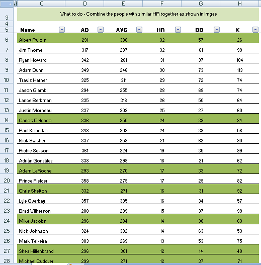
Great work was done by Mahesh! However, borders between non-repetitive values were also required (looks like we were expecting too much in 10 min). So the conditional formatting was not enough to win this activity.
There were multiple answers so Monika thought of using MS Excel to choose the next answer. She chose formula to pick the next answer sent by Jasdeep:
Jasdeep was about to hit the nail right on the head, but, he made a mistake by applying the formatting on all columns.
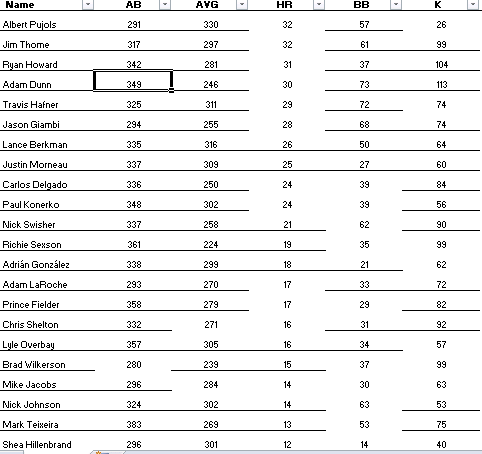
Next answer was from Krishna, and for this, he didn’t use the Choose formula. You dare not to ignore a solution sent by Krishna, whatsoever!Here is what Krishna had to say:
- First remove the borders from the cell range C6:H36
- Select these cells C6:H36, then select “New rule” in conditional formatting.
- Option for “Use a formula to determine which cells to format”, and put =$F6<>$F7 in the field “Format values where this formula is true”
- Click on format button, apply only “lower border”, and click OK
- Apply the created rule,
- Whoa!
What a comprehensive reply!! Kudos to you, Krishna! This was what Monika was looking for. Krishna was the winner of the activity!
I hope you also learned a new trick of Excel with us. Stay tuned. More activities like this will be coming in the future. We publish an activity every odd Saturday of a month. Set a reminder for the next odd Saturday. You have to visit this link: Click here
Authored by: Deepak Kumar, Research Analyst, Marketing Team